Classification Models belongs to the category of Supervised model, and should be used when we have to predict the target variable that is Categorical in nature, e.g.

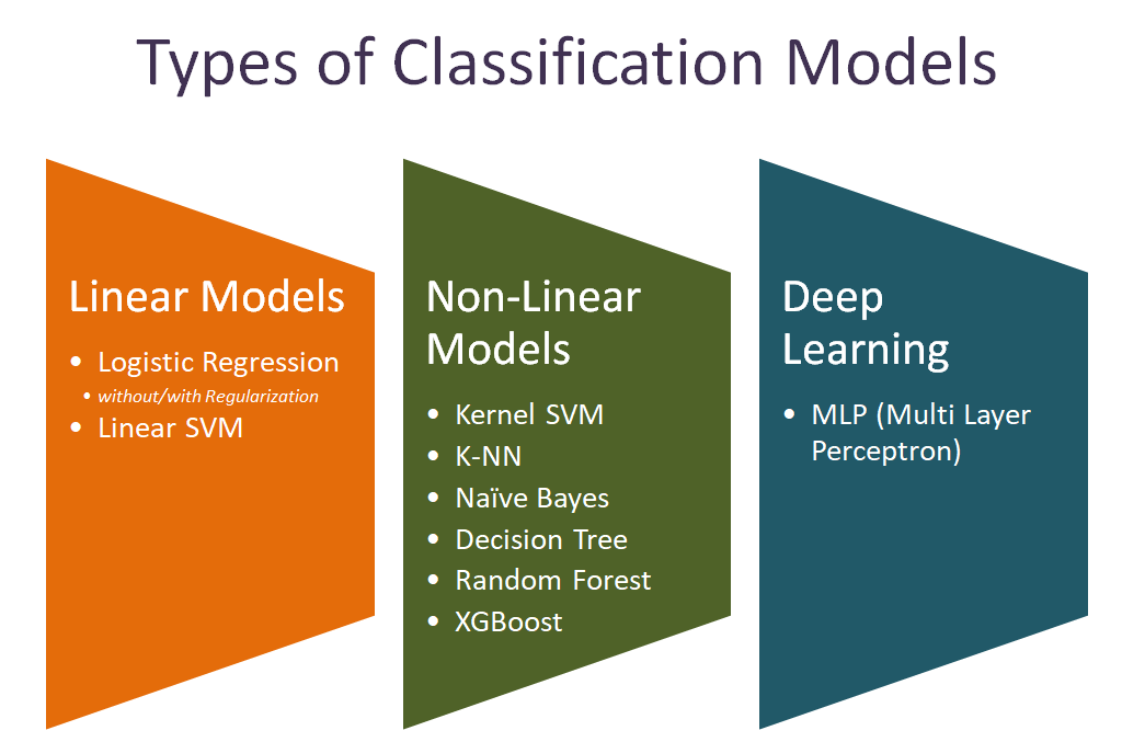
• There are two types of Classification
  1. Binomial – when target have 2 classes
  2. Multi-Class – when target have more than 2 classes

---

Here we will limit our discussion to Binomial Classification only

Refer below dataset where Target is Nominal Category i.e. 1 and 0, representing whether a Patient has Diabetes or Not. In such case we need to use Classification Models for ML.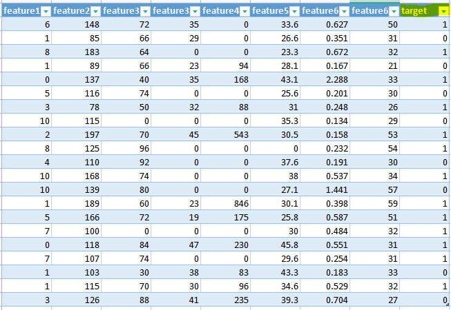

---

---

Logistic Regression Case Study

Its one of most important Classification Model that first computes the Decision Function using Linear Regression and then Applies Logistic Approach i.e. Sigmoid Function on top of that to limit the output between 0 and 1, that's why its known as Logistic Regression.

---

Step 1 : Apply Linear Regression

y = f(x) = m0 + m1*x1 + m2*x2  + …               
where m0 is intercept, m1 and m2 are slopes for x1 and x2 features resp.

*** y can range from (-infinity, +infinity)

-----------------------------------------------------------------

Step 2 : Apply Sigmoid Function

probability = 1/(1 + np.exp(-y))                   
where, np.exp is Numpy's Exponential Function

*** probability can range from [0,1]

---

Above chart shows the Sigmoid curve and its function/equation used in Logistic Regression

---

Python Program

First step is to load data using Pandas package

Then we do Data Cleaning and Feature Engineering

Next Important Step will be to check and solve for Class Imbalance Problem

# then we split data to TRAIN and TEST

from sklearn.model_selection import train_test_split


# Split dataset into training set and test set

X_train, X_test, Y_train, Y_test = train_test_split(data_X, data_Y, test_size=0.3,random_state=100)  

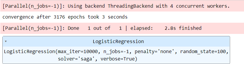
Training Phase Starts Here

# import the Python Class logistic regressor for CLASSIFICATION


from sklearn.linear_model import LogisticRegression



#creation of ML Model Object

classify = LogisticRegression(
    
    random_state=100, max_iter=10000, 
                              
    penalty='l1', solver='saga', 
                              
    verbose=True, n_jobs=-1
) 


# solver represents the actual algorithm to be used within the model e.g. sag [stochastic average gradient descent], saga [stochastic average gradient descent advance], lbfgs [limited memory-BFGS algo], etc.

# training starts here when the model learns the hidden data patterns by finding the best values for intercepts and coefficients by minimizing the Cost Function [i.e. Loss Function]


classify.fit(X_train, Y_train) 


#The Cost Function used in Logistic Regression is Log Loss [Binary Cross-Entropy].

#train accuracy score

classify.score(X_train,Y_train)

0.9118236472945892

Testing Phase Starts Here

Y_probability = classify.predict_proba(X_test)
print(Y_probability)

#it will print the predicted probabilities for class 0 [Negative class] and 1 [Positive class] respectively

array([
       [9.51647360e-01, 4.83526397e-02],
       [3.94828606e-01, 6.05171394e-01],
       [6.05822459e-02, 9.39417754e-01],
       [1.04476505e-01, 8.95523495e-01],
       [9.99498748e-01, 5.01251625e-04],
       [9.99997969e-01, 2.03093041e-06],
       [6.85487145e-02, 9.31451285e-01],
       [7.29609567e-02, 9.27039043e-01],
       ... and so on
      ])

Y_predicted = classify.predict(X_test)
print(Y_predicted)

#it will print the predicted class i.e. 0 or 1

array([
       0, 1, 1, 1, 0, 0, 1, 1, 0,
       1, 1, 0, 0, 1, 1, 1, 1, 1, 
       0, 0, 0, 1, 0, 0, 0, .....
      ])

# Test Accuracy

from sklearn import metrics


metrics.accuracy_score(Y_test, Y_predicted)

# Note that in Linear Regression, we used r2_score function

Error Analysis – Type 1 and Type 2 Errors

We need to first create the Confusion Matrix here

# TYPE 1 [False Positive] and Type 2 [False negative] ERRORs

from sklearn import metrics

print(metrics.confusion_matrix(Y_test,y_pred ))

[[98  6]
 [12 99]]

import seaborn as sns

sns.heatmap(metrics.confusion_matrix(Y_test,y_pred ),annot=True, fmt='d')

---

Confusion Matrix Explained in detail below:

---

from sklearn import metrics


print(metrics.classification_report(Y_test, y_pred))

---

ROC Curve – [Receiver Operating Characteristic]

AUC value [Area Under the Curve]

from sklearn import metrics

print(metrics.roc_curve(Y_test, y_pred))

#this will return 3 arrays:
# 1. FPR [False Positive Rate]
# 2. TPR [True Positive Rate]
# 3. Thresholds

(
 array([0., 0.05769231, 1.]), 
 array([0., 0.89189189, 1.]), 
 array([2, 1, 0])
)

fpr = [0., 0.05769231, 1.]
tpr = [0., 0.89189189, 1.]

#ROC CURVE

import matplotlib.pyplot as plt
plt.scatter(fpr, tpr)
plt.plot(fpr, tpr)

#guess line [Random Classifier]
plt.plot([0,1],[0,1])
plt.show()

#Test Accuracy - function 1

print(metrics.auc(fpr, tpr))

0.9182103599999999

#Test Accuracy - function 2

print(metrics.roc_auc_score(Y_test, y_pred))

0.9170997920997921

---

CONCLUSION:

From the above steps/calculations, we found that --

Train Accuracy - 0.9118236472945892

Test Accuracy using accuracy_score function - 0.9162790697674419
Test Accuracy using confusion matrix function - 0.916 [(TP+TN)/Total]
Test Accuracy using ROC and AUC function - 0.9182103599999999 and 0.9170997920997921

***Hence, this Seems to be a Good Fit/Model for the given dataset here.

---